From individual incidents to statistically significant spatial patterns.
This project examines how reported motor vehicle crime patterns change when the same incident dataset is analyzed through administrative aggregation, continuous density, local spatial statistics, and transportation proximity.
A list of 15,149 mapped record locations does not, by itself, reveal where a city's motor vehicle crime pattern is concentrated. This independent GIS research project builds a connected six-map workflow in ArcGIS Pro 3.6 that answers that question from four distinct analytical angles: how incidents are distributed once summarized to police districts and neighborhoods, where continuous concentration is elevated regardless of boundaries, where clustering is statistically significant rather than simply visually dense, and how closely incidents fall to San Francisco's major-road network.
Analytical layers were standardized in NAD 1983 UTM Zone 10N (EPSG:26910), providing a consistent projected coordinate system for density, spatial-statistics, and distance workflows. The project combines data preparation, spatial analysis, cartography and technical reporting in six maps and a revised 33-page report. Map 05 now shows FDR-corrected results; the other five map images are unchanged. Remaining provenance checks are stated explicitly.
Key Findings
What four analytical methods show about the same dataset.
Each finding below comes from a different spatial method. Read together, not in isolation, they form the project's central analytical argument.
Incident Distribution
15,149
Mapped motor vehicle crime records were included in the analytical dataset, San Francisco, 2021–2025. Unique-event identifiers remain a provenance check.
Administrative Aggregation
2,599
Bayview recorded the highest displayed police-district total, followed by Ingleside (2,212) and Mission (2,088). Full district breakdown in Map 02 below.
Density & Hot Spots
Central / NE
FDR-corrected Gi* identifies 314 hot-spot cells concentrated in central and eastern San Francisco, including parts of Bayview. Only two cold-spot cells remain, both at 90% confidence.
Density and statistical significance answer different questions. Map 05 now uses FDR correction; the other five map images are unchanged.
Road Proximity
58.7%
Of mapped records fell within 250 m of the nearest major road (30.2% within 100 m; 28.5% between 101–250 m).
A spatial association, not a causal claim.
Analytical Story
Six maps, one incident dataset, four spatial questions.
The series moves from raw incident points to administrative aggregation, continuous density, statistically significant clustering, and transportation proximity — each method answering a distinct research question. Select any map to view it enlarged.
01Baseline Map
Incident Distribution
Question
Where are reported incidents located?
Method
Point feature visualization of all 15,149 mapped records against police-district and city-boundary context layers.
View full map ↗
What it shows
Incidents are distributed throughout the city but are more densely packed in central, northeastern, and southeastern areas, with western districts showing a more dispersed pattern.
Why it matters
Establishes the raw spatial baseline before any aggregation, smoothing, or statistical modeling is applied.
Point MappingCartographic Design
02Administrative Aggregation
Motor Vehicle Crime by Police District
Question
How do incident totals vary across police districts?
Method
Spatial Join of incident points to the ten SFPD district polygons, classified with five-class Natural Breaks (Jenks).
View full map ↗
Displayed District Totals
Bayview2,599
Ingleside2,212
Mission2,088
Northern1,704
Southern1,589
Taraval1,529
Central1,197
Richmond776
Park775
Tenderloin674
Interpretation
These are raw mapped incident counts, not population-normalized crime rates. Districts vary in size, land use, and street density, so totals should be interpreted alongside neighborhood, density, and hot-spot results — not as a standalone risk measure.
Spatial JoinNatural Breaks (Jenks)
03Administrative Aggregation
Motor Vehicle Crime by Neighborhood
Question
What finer-scale spatial variation appears when incidents are summarized by neighborhood instead of police district?
Method
A second Spatial Join aggregates the same incidents to San Francisco's neighborhood polygons, again classified with five-class Natural Breaks (Jenks).
View full map ↗
Why geography matters. Changing the aggregation unit reveals local variation that can be obscured by larger police-district boundaries — a practical example of the Modifiable Areal Unit Problem: the same events can look different depending on the boundaries used to summarize them.
Why it matters
Demonstrates that administrative results are scale-dependent, not a fixed property of the underlying data.
Spatial JoinNatural Breaks (Jenks)
04Continuous Density
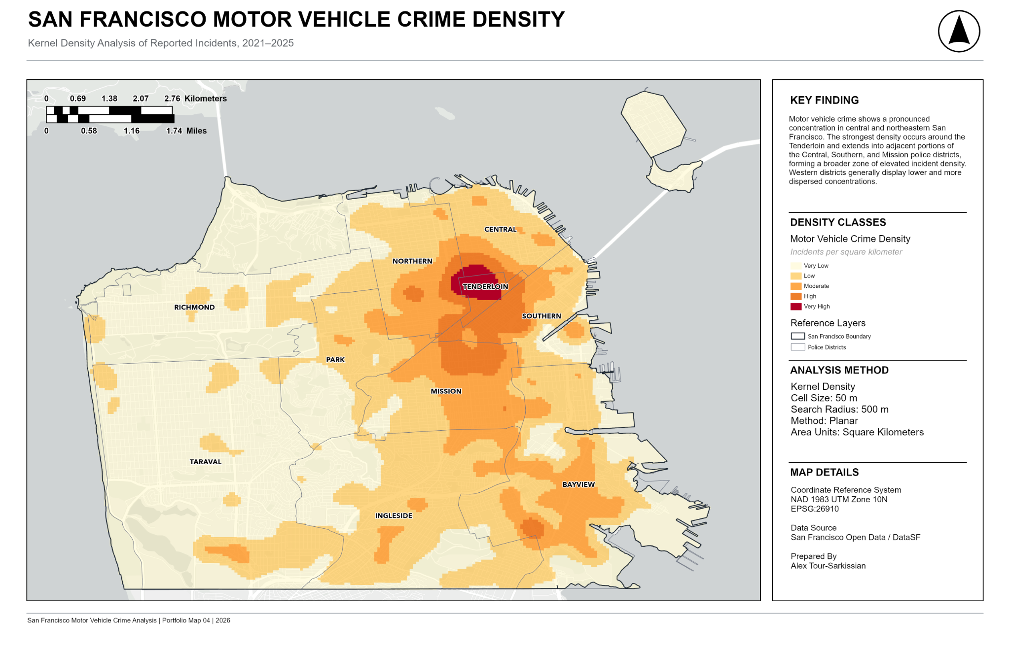
Motor Vehicle Crime Density
Question
Where does incident concentration remain high regardless of administrative boundaries?
Method
Kernel Density estimation over the mapped incidents, masked to the San Francisco boundary.
View full map ↗
50 mCell Size
500 mSearch Radius
PlanarMethod
km²Area Units
What it shows
The strongest continuous concentration is centered around Tenderloin and extends into adjacent portions of Central, Southern, and Mission; western districts are generally lower and more dispersed.
Density models concentration on a continuous surface. It is not a statistical-significance test and should not be read as a probability or causal surface.
Kernel DensityRaster Analysis
05Statistical Clustering
Motor Vehicle Crime Hot Spots
Question
Where does statistically significant spatial clustering occur — as distinct from cells that are simply high in value?
Method
FDR-corrected Getis-Ord Gi* on 3,066 fishnet cells; Join_Count; fixed 400 m band; Euclidean distance.
View full map ↗
90%Confidence
95%Confidence
99%Confidence
What it shows
FDR-corrected analysis identifies 314 hot-spot cells in central and eastern San Francisco, including parts of Bayview. Only two cold-spot cells remain, both at 90% confidence; 2,750 cells are not statistically significant.
The corrected hot-spot total includes 225 cells at 99%, 66 at 95% and 23 at 90%. Broad western cold spots from the earlier uncorrected output are not retained. Gi* classifications describe clustering under the specified model, not population-adjusted risk or causes.
Getis-Ord Gi*Spatial Statistics
06Proximity Analysis
Motor Vehicle Crime Near Major Roads
Question
How close are mapped incidents to San Francisco's major-road network?
Method
Near analysis (planar distance) from each incident to the nearest major road, classified into distance bands.
View full map ↗
58.7%Within 250 m
30.2%0–100 m
28.5%101–250 m
20.9%251–500 m
20.4%>500 m
This identifies a spatial association and a transportation-corridor pattern worthy of further investigation — it does not demonstrate that roads cause motor vehicle crime.
Near AnalysisBuffer Analysis
Methods & Workflow
From raw records to interpretable spatial evidence.
Each stage is a discrete, checkable step in ArcGIS Pro 3.6, moving from descriptive mapping toward increasingly transformed spatial representations.
01
Acquire & review source data
Reviewed SFPD incident reports published through DataSF and municipal boundary, police-district, neighborhood, and road reference layers.
02
Prepare incident records
Filtered the broader incident source to the 2021–2025 motor vehicle crime subset and retained the fields needed for analysis.
03
Validate geometry and attributes
Reviewed field names, null values, and geographic attributes; separated authoritative base layers from derived analytical outputs.
04
Project analysis layers to NAD 1983 UTM Zone 10N
Standardized all distance- and density-based analysis in EPSG:26910 so results are measured in consistent meter units.
05
Aggregate incidents by administrative geography
Ran Spatial Join against police districts and neighborhoods; classified results with five-class Natural Breaks (Jenks).
06
Model continuous density
Generated a Kernel Density surface at 50 m cell size and 500 m search radius, masked to the San Francisco boundary.
07
Test local spatial clustering
Built a crime-analysis fishnet and ran Gi* on cell counts. The October 21 audit reproduced earlier statistics with a fixed 400 m Euclidean band, then applied FDR correction and updated Map 05.
08
Measure proximity to major roads
Ran Near analysis on a derived analysis copy, classified NEAR_DIST into distance bands, and summarized percentages with Summary Statistics.
09
Validate analytical outputs
Reconciled the district difference, checked fishnet counts and reproduced earlier exported Gi* statistics before comparing FDR classes. Original extraction, neighborhood provenance and road-distance class logic remain separate checks.
10
Design and export final cartographic products
Applied a consistent portfolio layout — legend, north arrow, dual-unit scale bar, key finding — across all six final maps.
Analytical Parameters
Configuration, not just button-clicking.
Each analytical method depends on configuration choices that shape the resulting output. Documenting them here supports reproducibility and technical review.
Checking the analysis instead of assuming the output is correct.
The October 21, 2026 audit reconciled district assignments, checked fishnet counts and compared reproduced Gi* output with FDR-corrected classes.
Verification audit: 15,143 of 15,149 mapped records intersect one district; six records at four locations intersect none, and zero intersect multiple districts. Near distances are approximately 0.10–22.07 m. No points were moved and source-coded districts were retained; the check does not establish which geometry is inaccurate. The 3,066 fishnet cells sum to 15,143, including 981 zero-count cells, with counts 0–108 and no null or negative counts. Matching totals alone does not establish that the same six records were excluded from both. Matching SOURCE_ID reproduced the earlier exported counts, neighbors, z-scores, p-values and bins exactly at export precision using a fixed 400 m Euclidean band with FDR off; this does not recover the original execution log. Compared with that historical no-FDR output, FDR correction changes hot cells from 471 to 314, cold cells from 564 to two, and non-significant cells from 2,031 to 2,750. Across matched features, 810 bins change while counts, neighbors and raw z-scores/p-values remain unchanged; raw p-values are not FDR-adjusted p-values.
Geometry review
Attribute review
Coordinate-system verification
Projected-distance validation
Spatial-join count checks
Summary-statistics review
Raster-output inspection
Gi* output review
Near-distance review
Map-layout review
Cross-method interpretation
Interpretation
One dataset. Different spatial questions.
The same 15,149 records produce four different — and complementary — analytical answers, depending on the method used to examine them.
Administrative Counts
Where are incidents assigned once summarized to a police district or neighborhood boundary?
Density
Where is incident concentration elevated continuously across space, independent of any boundary?
Statistical Clustering
Where are high or low spatial values clustered more strongly than the selected spatial model would expect by chance?
Proximity
How close are mapped incidents to San Francisco's major-road network?
Counts ≠ Density ≠ Statistical Hot Spots ≠ Proximity
Methodological Scope & Limitations
What this project demonstrates — and what it doesn't.
This project demonstrates a retrospective, descriptive and exploratory spatial analysis of publicly available motor vehicle crime data: administrative aggregation, continuous density estimation, local spatial statistics, and transportation-proximity analysis in ArcGIS Pro, with documented QA/QC throughout.
Incident locations reflect the source data's reporting, geocoding, and privacy-protection practices (DataSF maps incidents to nearby intersections rather than exact coordinates).
DataSF's incident-location mapping process changed on April 24, 2024, which should be considered when interpreting fine-scale spatial patterns across the full 2021–2025 study period.
Police-district and neighborhood totals are raw mapped incident counts, not population-normalized crime rates.
Administrative aggregation results depend on the boundaries used to summarize incidents and will change if those boundaries change.
Kernel Density output depends on the selected cell size and search radius.
Getis-Ord Gi* depends on grid geometry, spatial relationships and multiple-testing correction. Map 05 uses FDR; extensive western cold spots are not retained. Exact source identifiers, offense/date filters, neighborhood provenance and road-distance class logic remain outstanding. The reported 58.7% road-proximity share is descriptive, not a newly revalidated excess-risk finding.
Road-proximity analysis identifies spatial association, not causation.
This is retrospective, descriptive and exploratory spatial analysis — it is not predictive policing and not a live public-safety system.
It should not be interpreted as an assessment of individual people or of any specific neighborhood.
It is an independently produced research project. It is not a claim of employment by the City of San Francisco, work commissioned by DataSF, or deployment by the San Francisco Police Department.
Full Report
Explore the full GIS research report.
The revised 33-page report includes the corrected Figure 5, district reconciliation and October 21 Gi* reconstruction/FDR comparison. Appendix B records the verification results, chronology and remaining provenance checks.
This project demonstrates an end-to-end GIS workflow: preparing and validating spatial data, managing projected coordinate systems, performing vector and raster analysis, applying spatial statistics, validating analytical outputs, designing professional cartography, and communicating defensible findings and limitations.
Data Preparation & QA/QC
Preparing spatial data for analysis, validating geometry and attributes, checking coordinate systems, and reconciling analytical outputs against source totals.
Spatial Data PreparationCoordinate SystemsQA/QCSummary Statistics
Spatial Analysis
Using vector, raster, aggregation, and proximity methods to answer distinct geographic questions from the same incident dataset.
Distinguishing descriptive spatial concentration from statistically significant clustering and documenting the parameters used to interpret each result.
Kernel DensityGetis-Ord Gi*Spatial Statistics
Cartography & Communication
Turning analytical outputs into consistent professional map products, explaining results clearly, documenting limitations, and communicating findings without overstating what the analysis supports.
ArcGIS ProCartographic DesignTechnical DocumentationAnalytical Communication
GIS Analysis · Spatial Statistics · Cartography
Explore the complete methodology and technical documentation, or continue to my GIS experience and project work.